
Press release · 15 November 2026 · version 0.1.0-candidate
Quantile and threshold calibration separate even for Gaussian forecasts
Passing every quantile calibration check does not mean passing every threshold check, even for smooth Gaussian forecasts: the two checks weight the same probability-zero set of forecasts differently, and errors reach about one percentage point.
Summary
In one sentence. Two standard ways of checking whether probabilistic forecasts are calibrated, quantile checks and threshold checks, can give opposite verdicts even for smooth Gaussian forecasts, so passing one does not certify the other.
The everyday problem. Many forecasts are probability distributions rather than single numbers: a weather service's spread of possible temperatures, a central bank's fan chart for inflation, a machine-learning model's predictive distribution for a house price. Such a forecast is calibrated if its probabilities can be taken at face value: of all the days on which it says "10% chance of more than 30 degrees", about 10% should be hotter than that.
Two standard checks. A threshold check fixes a value, say 30 degrees, groups the forecasts by the chance they give of staying below it, and asks whether those chances match what happened (threshold reliability diagrams display this). A quantile check fixes a probability, say one half, groups the forecasts by their median, and asks whether outcomes fall below the forecast median half of the time (conditional exceedance probability checks do this at every level).
Why they look identical. For a smooth forecast, "the chance of staying below 30 is 50%" and "the median is 30" pick out exactly the same forecasts. So passing every quantile check should mean passing every threshold check, and the reverse.
What was known. Gneiting and Resin (2023) proved the equivalence when the forecast can take only countably many different shapes, conjectured that this restriction could be dropped, and noted that under technical conditions the two kinds of test assess identical hypotheses. A recent overview by Resin, Yang and Gneiting (2026) still draws these implications as conjectures, together with four more for unordered categories.
What is new here.
| Setting | Result | Where |
|---|---|---|
| Smooth Gaussian forecasts | Countability cannot be dropped: one outcome law passes every quantile check exactly, with a perfectly flat PIT histogram, yet fails every threshold check; another does the reverse. Errors reach about one percentage point | Theorem 3.1, Section 3.5 |
| Outcomes with $k$ ordered categories | The quantile-type check implies the threshold check if $k\le3$ or the forecast takes countably many shapes; it can fail for $k\ge4$ | Theorems 4.1–4.3 |
| Unordered categories | Checking the PIT under every ordering guarantees the category frequencies, with a sharp bound; class-wise calibration does not guarantee average probabilistic calibration; two further implications are settled for up to three classes and stay open beyond | Section 5 |
| Any smooth forecast family | The general identity relating the two checks, a bound on how far they can differ, and a local construction | Sections 6–7 |
A concrete example. With perturbation size $\varepsilon=1/10$, outcomes in the first example fall below zero $50.76\%$ of the time while the forecasts say $50\%$ on average. A standard binomial test at the $5\%$ level with $80\%$ power needs about $34{,}000$ forecast cases to detect this: an ordinary verification sample.
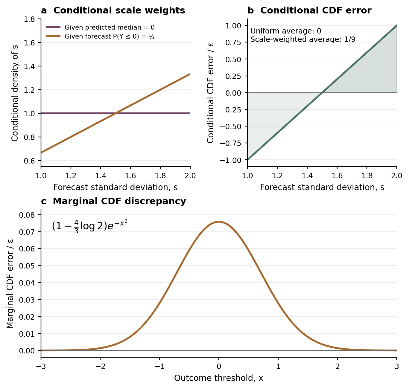
Why it happens. Forecasts with "median $=0$" and forecasts with "chance below $0$ is $50\%$" are the same set. But that set has probability zero, and the two checks weight its members differently: the quantile check evenly, the threshold check in proportion to the forecast's spread. An error that averages to zero under one weighting averages to $1/9$ (times $\varepsilon$) under the other. This is the classical Borel–Kolmogorov paradox: conditioning on an event of probability zero depends on how the event is described. When forecasts take countably many shapes, every relevant event has positive probability and the paradox disappears.
Practical message. When forecasts vary continuously, as they do for parametric and machine-learning regression models, run both kinds of check: passing one does not certify the other.
Limits. These are constructed population examples, not a study of any real forecasting system. The perturbation size $1/10$ rests on a computer-assisted interval-arithmetic bound; the analytic proof alone gives $1/400$. Two implications for unordered categories remain open for four or more classes. Statistical tests with finite samples are not studied. This is an unrefereed candidate; its assurance is internal AI-assisted review and computational checks, not peer review.
Summary for specialists
A prediction space has a random forecast CDF $F$ and outcome $Y$; $Z$ is the randomised PIT. CC: $P(Z\le\alpha\mid F^{-1}(\alpha))=\alpha$ (conditional exceedance probability calibration); QC: conditional quantile calibration; TC: $P(Y\le x\mid F(x))=F(x)$; MC: $P(Y\le x)=E F(x)$; PC: $Z$ uniform.
- Theorem 3.1 (proof): let $M\sim U[-1,1]$ and $S\sim U[1,2]$ be independent and issue $F=\Phi((x-M)/S)$. With $\psi=(1-m^2)(s-1)(2-s)$, $\chi(x)=e^{-x^2}$ and $K=z\,\partial_m\psi-\partial_s\psi$, $z=(x-m)/s$, the laws $G^Q=F+\varepsilon\chi K$ and $G^T=F+\varepsilon\chi K/s$ are CDFs with densities in $[f/2,3f/2]$ for $0<\varepsilon\le1/10$. Under $G^Q$: CC, QC and PC hold, TC and MC fail at every threshold, and $P_Q(Y\le x)-E F(x)=\varepsilon c_0e^{-x^2}$ with $c_0=1-\tfrac43\log2$. Under $G^T$: TC and MC hold, CC and QC fail at every level, and $P_T(F(Y)\le\alpha)<\alpha$ for all $\alpha\in(0,1)$.
- Theorems 4.1 and 4.2 (proof): for $k$ ordered outcome values with positive forecast probabilities, CC implies TC if the forecast has countable support (any $k$) or $k\le3$ (any law).
- Theorem 4.3 (proof): an explicit four-value forecast, with one continuous parameter and positive probabilities, satisfies CC, PC and MC but fails TC at threshold 2; the error at $F_2=1/2$ is $1/640$.
- Theorems 5.3 and 5.5, Corollary 5.1, Proposition 5.6 (proof): for nominal outcomes, fPC implies MC, and the marginal error in total variation is at most $2d-d^2$, sharp, where $d$ bounds the Kolmogorov distance of every ordered PIT from uniform; fCC $\Rightarrow$ fTC and pCC $\Rightarrow$ pTC hold for $k\le3$ or countable support; CwC does not imply aPC, with all probabilities positive.
- Theorem 6.1 (proof): in a location–scale family, a compactly supported perturbation $R$ preserves CC exactly when $R=\mathsf D_x\vartheta$, TC exactly when $R=s^{-1}\mathsf D_x\vartheta$, and both exactly when $R=\mathsf D_x^2\eta$, for compactly supported potentials, where $\mathsf D_x=z\,\partial_m-\partial_s$.
- Theorem 7.1 and Proposition 7.2 (proof): on a common fibre the threshold- and quantile-conditional parameter laws differ by the factor $f_\theta(x)$; the two conditional means agree for all outcome laws only if $f_\theta(x)$ is constant on the fibre, and otherwise differ by at most $(\sqrt\Lambda-\sqrt\lambda)/(\sqrt\Lambda+\sqrt\lambda)$ when the density ratio lies in $[\lambda,\Lambda]$.
Table 2 of the paper lists the status of every conjectured implication in the hierarchies of Gneiting and Resin (2023) and Resin, Yang and Gneiting (2026).
Technical account
Two weightings of one segment. Fix a level $\alpha$ and put $z_\alpha=\Phi^{-1}(\alpha)$. The forecasts with $\alpha$-quantile $t$ and the forecasts with $F(t)=\alpha$ form the same segment $\{(t-sz_\alpha,s)\}$ in parameter space. Given the quantile, $S$ is uniform on the segment; given the threshold probability, $S$ has density proportional to $s$ (Lemma 3.3). Along the segment the error $K(t-sz,s,t)$ is minus the derivative of $\psi(t-sz,s)$ in $s$, and $\psi$ vanishes at the ends, so the uniform average is zero: CC and QC hold under $G^Q$. Under the scale weight the same error has a strictly positive average; dividing by $s$ (the law $G^T$) swaps the roles.
Effect sizes. On the segment $t=0$, $\alpha=1/2$, the error is $\varepsilon(2s-3)$: it averages to $0$ uniformly and to $\varepsilon/9$ under the weight $2s/3$, as Figure 1 shows. Averaged over all forecasts, $G^Q$ leaves the marginal discrepancy $\varepsilon c_0e^{-x^2}$. At $\varepsilon=1/10$ the quantile error of $G^T$ on the same segment is $\varepsilon(2-3\log2)\approx-0.0079$, and its PIT distribution function at $1/2$ is $0.49557$.
The amplitude certificate. Validity of the outcome laws needs $\varepsilon\,|\partial_xB|\le f/2$. An analytic envelope gives $\sup|\partial_xB|/f<113$, hence $\varepsilon\le1/400$. The script certify_amplitude.py bounds the ratio by $5$ on $[-1,1]\times[1,2]\times[-6,6]$ in outward-rounded interval arithmetic, bisecting boxes until each is accepted; the tail $|x|>6$ is analytic. This gives $\varepsilon\le1/10$. The true suprema are about $4.82$ and $4.69$.
Finitely many outcome values. For a step forecast the PIT error interpolates linearly between consecutive cumulative residuals, so CC becomes a family of averaged identities. With countable support, the jumps of these averages recover TC threshold by threshold; with $k\le3$, the first and last thresholds are all there are. With four values, CC constrains the middle residual only through averages over random intervals. The construction in Theorem 4.3 uses commuting averaging operators to make those averages vanish while the conditional mean given $F_2$ does not. The script checks this in exact rational arithmetic.
Nominal outcomes. Rotating a block of classes from the front of an ordering to the back changes the PIT by exactly $\mathbf 1\{Y\in A\}-P(A)$. If every ordering gives a uniform PIT, both orderings have PIT mean $1/2$, so $P(Y\in A)=E P(A)$. A Kolmogorov-distance bound on the PIT mean gives the sharp stability bound $2d-d^2$.
Evidence, assurance and limitations
The synthetic audio briefing is explanatory, not additional evidence. Its complete transcript is available for reading.
- Proofs. Every result has a written proof in the 20-page paper. The paper opens with a plain introduction and a roadmap; Section 8 lists consequences and limits. No proof assistant was used.
- Computational checks.
verify_gaussian.pychecks the symbolic identities, the constant $c_0$, the segment values $\varepsilon/9$ and $\varepsilon(2-3\log2)$, conditional errors computed directly from the joint law by quadrature, strict signs at many levels, the effect sizes and the sample size.verify_discrete.pychecks Theorem 4.3 in exact rational arithmetic, the discrete implications by rank tests on grid laws, the block-rotation identity, the extremal laws and both nominal counterexamples.certify_amplitude.pyis the interval certificate, the one computer-assisted step of a proof. - Tests that can fail. No script uses
assert, so the checks stay active under Python's optimised mode. Lowering the certified bound to $4.7$, below the true supremum, or swapping two table entries of the four-value construction makes the scripts fail underpython -O, as they must. - Replay. All three scripts were rerun from fresh copies before release, normally and under
python -O, with pinned numpy, scipy, sympy and mpmath; every recorded output was reproduced byte for byte. GitHub CI reruns the exact checks, the certificate and both negative controls on Linux as a blocking job, and the Gaussian checks as a non-blocking job. - Review. Five internal AI-assisted reviewer roles, an adversarial review by a second AI model and a clean replay found no mathematical error and led to one revision round. It added a plain introduction, stated the conjectures from the sources, certified the larger amplitude with effect sizes, explained the consequences for testing, and added the discrete boundary, the nominal results and the status table. A re-review, a proof audit and a second-model audit of the new proofs found no failing theorem and led to precise wording corrections. A rating-free summary is in the package. None of this is peer review, independent reproduction or formal verification.
- Limitations. Population constructions; no deployed forecast system was studied. The amplitude $1/10$ rests on the interval certificate; the analytic proof gives $1/400$. The nominal implications fCC $\Rightarrow$ fTC and pCC $\Rightarrow$ pTC remain open for four or more classes with uncountable forecast families. Finite-sample tests, and the largest threshold error compatible with exact quantile calibration, are not treated. Attributions rest on a bounded literature search. This remains an unrefereed candidate.
Who should care, and why
| Audience | Potential use | Required caution |
|---|---|---|
| Forecast verification teams (weather, economics, machine learning) | Evidence that quantile-type and threshold-type checks test different things when forecasts vary continuously, so both should be run | Constructed examples; no estimate of error in any deployed system |
| Developers of calibration diagnostics and tests | Explicit separating laws for testing a diagnostic, and the reweighting identity that converts one target into the other | Finite-sample behaviour of tests is not studied |
| Researchers on calibration hierarchies | The status of every conjectured arrow in the Gneiting–Resin and Resin–Yang–Gneiting hierarchies | Two nominal implications stay open for four or more classes |
| Research agents | Machine-readable claims, an agent index and replayable scripts | Except for the certificate, the scripts are checks, not proofs |
Why the problem matters
Reliability diagrams, PIT histograms and conditional exceedance tests are routine in weather, economic and machine-learning forecast verification. Practitioners have been told, under technical conditions, that quantile-type and threshold-type tests assess the same hypothesis, and they often run only one. For forecasts whose parameters vary continuously with covariates, which is the usual case for regression models, this paper shows that the hypotheses differ, by errors large enough to matter in ordinary samples. It also locates exactly where the published equivalence stops for outcomes with a few ordered categories.
How to inspect or reproduce the recorded checks
From the GitHub release or the Zenodo archive, from a directory outside the package (Python 3.12 with the pinned packages in requirements.txt):
V=/absolute/path/to/package/verification
shasum -a 256 -c MANIFEST.sha256          # at the package root
python3 -m pip install numpy==2.3.5 scipy==1.17.0 sympy==1.14.0 mpmath==1.3.0
python3 -O -I -B "$V/verify_gaussian.py" --out /tmp/qtc
python3 -O -I -B "$V/verify_discrete.py" --out /tmp/qtc
python3 -O -I -B "$V/certify_amplitude.py" --out /tmp/qtc
ENVIRONMENT.txt lists the software used. AI_INDEX.md maps each claim to its proof and checks, RESEARCH_GATES.json gives the prior-work boundary, and REVIEW_SUMMARY.md lists the review objections and how each was handled.
The most valuable next projects
- Settle fCC $\Rightarrow$ fTC and pCC $\Rightarrow$ pTC for four or more nominal classes with uncountable forecast families.
- Find the largest threshold error compatible with exact quantile calibration, and the converse.
- Study the power of binned exceedance and threshold tests against these alternatives in finite samples.
- Measure the gap between the two kinds of check in real verification data sets.
What is in the evidence package
The paper (LaTeX source and PDF, with Figure 1 and its script); verification/verify_gaussian.py, verification/verify_discrete.py, verification/certify_amplitude.py and their recorded outputs; requirements.txt; refs.bib from Crossref and arXiv records; AI_INDEX.md; REVIEW_SUMMARY.md; RESEARCH_GATES.json; REPLAY_RECEIPT.md and ENVIRONMENT.txt; citation metadata, licences (CC0-1.0 for text, figures and data, MIT for code), the CI workflows and SHA-256 sums.
Verification status
Unrefereed AI-assisted mathematics candidate with written proofs and one computer-assisted interval certificate. Internal AI-assisted review in five reviewer roles and an adversarial review by a second AI model, clean replays, one revision round with extensions (the certified amplitude and effect sizes, the boundary for finitely many ordered outcome values, the nominal results merged from a companion note, the status table), then a re-review, a proof audit and a second-model audit of the new proofs; no mathematical error was found, and summary wording was corrected. Except for the amplitude certificate the scripts are checks, not proofs. External specialist review, independent reproduction and formal verification have not been established.
Cite
BibTeX
@misc{quantilethresholdcalibrationseparate2026,
  title        = {Quantile and threshold calibration separate even for Gaussian forecasts},
  author       = {Anonymous},
  year         = {2026},
  doi          = {10.5281/zenodo.24259222},
  url          = {https://doi.org/10.5281/zenodo.24259222},
  version      = {0.1.0-candidate},
  howpublished = {Zenodo},
  note         = {Unrefereed; internally replayed evidence package. Press page: https://evidencepress.org/releases/quantile-threshold-calibration-separate/}
}Also: cite.bib · paper.json · this page as Markdown