
Press release · 4 November 2026 · version 0.1.0-candidate
Compact completion and uniform statistical bounds for hyperbolic geodesic sliced Wasserstein distance
Geodesic sliced Wasserstein distance on hyperbolic space is exactly a weak-convergence metric on the compact closed Klein ball: it has an exact diameter, barely sees depth far from the centre, gives squared distance π·α between boundary points at angle α in two dimensions, and can be estimated at optimal rates with no assumptions on the data.
Summary
The setting. Data with a tree-like or hierarchical shape (family trees, word hierarchies, citation and social networks) are often embedded in hyperbolic space, a geometry in which the room available grows exponentially as you move away from the centre. Machine-learning methods then need to compare two clouds of embedded points. Optimal transport (the Wasserstein distance) does this well but is expensive. Sliced Wasserstein distance makes it cheap: project both clouds onto many lines through a fixed centre, compare them on each line, where the problem is easy, and average. Bonet and co-authors (2023) introduced the version that projects along hyperbolic geodesics through the centre. It is used as a training loss and as a way to compare distributions.
The question. What does this distance actually measure? A small value should tell a user something definite: which kind of convergence it detects, which space of distributions it lives on, and how accurately it can be estimated from data.
The answer. In the Klein picture of hyperbolic space (a ball whose straight chords are the geodesics), each projection is simply $\operatorname{atanh}(v\cdot z)$. These projections stay bounded on average even at infinity. Everything follows from that.
- It lives on the closed ball (proved). The distance extends to distributions on the closed ball, boundary sphere included, which is compact. Mass that drifts off to infinity converges to the boundary instead of escaping. The distance has an exact maximum value, detects ordinary (weak) convergence, and cannot see how heavy the far tails are.
- It barely sees depth (proved). Two points far out in the same direction are exponentially close in this distance, however far apart they really are. In the plane with quadratic loss, points at hyperbolic depth 4 and 8 on one ray are only about 0.21 apart, and a point's distance from the centre levels off at $\pi/2$.
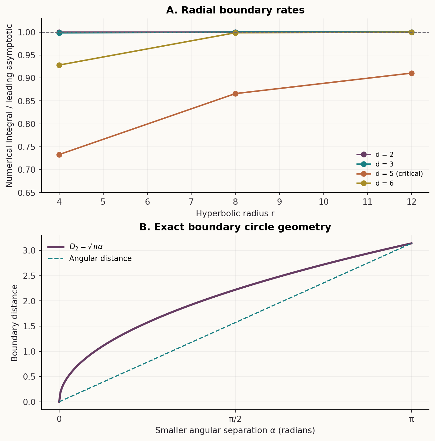
- The boundary sphere has an exact geometry (proved). In two dimensions the squared distance between two points at infinity is exactly $\pi$ times the angle between them. In three dimensions it behaves like $\tfrac12\alpha^2\log(1/\alpha)$ for small angle $\alpha$; from four dimensions on it is comparable to $\alpha^2$, with an exact constant.
- A published claim is corrected (proved). Proposition 19 of Bonet, Drumetz and Courty (JMLR 2025) says that a certain back-projection vanishes at infinity. A simple explicit function shows that it does not.
- Estimation needs no assumptions (proved). The distance between a sample of size $n$ and its population shrinks like $n^{-1/2}$ (for the powered loss) for every distribution, with no moment or support conditions, in expectation and with high probability, and this rate cannot be improved.
- A cheap repair (proved). Adding one comparison of the distributions of distances from the centre gives a complete metric with the usual hyperbolic Wasserstein convergence.
The sections below move from this overview to a specialist summary, the technical argument, evidence and limits, and how to rerun the checks.
Summary for specialists
Let $G_v(x)$ be the signed geodesic projection of $x\in\mathbb H^d$ onto the geodesic through a fixed origin $o$ in direction $v\in S^{d-1}$, and $\operatorname{GHSW}_p(\mu,\nu)^p=\int_{S^{d-1}}W_p^p((G_v)_\#\mu,(G_v)_\#\nu)\,d\sigma(v)$ (Bonet et al. 2023). Let $C_{d,p}$ be the $p$th absolute moment of the density $c_d\operatorname{sech}^{d-1}t$; $C_{d,2}=\tfrac12\psi_1(\tfrac{d-1}2)$. Results, for $d\ge2$ and $1\le p<\infty$:
| Result | Statement in brief | Where |
|---|---|---|
| Completion | $\operatorname{GHSW}_p$ extends to $D_p$ on $\mathcal P(\overline B^d)$, its compact completion; weak topology; no moment assumption | Thm 2.3 |
| Diameter | exactly $2C_{d,p}^{1/p}$ | Thm 2.3 |
| Correction | the $C_0$ backprojection claim of Bonet, Drumetz and Courty (Prop. 19) fails: $g=\operatorname{sech}^2t$ gives $1-\tanh^2r/d\to1-1/d$ | Prop 3.1 |
| Radial rates | $e^{-(d-1)r}$, $re^{-2pr}$, $e^{-2pr}$ as $d-1<,=,>2p$, exact constants | Thm 4.1 |
| Depth insensitivity | far points on one ray are exponentially close | Cor 4.2 |
| Boundary geometry ($p=2$) | $\pi\alpha$ ($d=2$); $\tfrac12\alpha^2\log\tfrac1\alpha$ ($d=3$); $\asymp\alpha^2$, limit $\frac{d-2}{(d-1)(d-3)}$ ($d\ge4$) | Prop 4.3, Thm 4.4 |
| Sampling | $\mathbb E D_p^p(P_n,P)\le S_{d,p}n^{-1/2}$ for every $P$; high-probability version | Thm 5.1 |
| Minimax | rate $n^{-1/2}$ for $D_p^p$ and $n^{-1/(2p)}$ for $D_p$; constants not sharp | Thm 5.2, Cor 5.3 |
| Augmentation | $\mathcal D_p=(\operatorname{GHSW}_p^p+W_p^p(\text{radial laws}))^{1/p}$ is complete with the $W_p^{\mathbb H}$ topology | Thm 6.1 |
| Finitely many directions | never separate laws, even with the radial law | Prop 6.2 |
Attribution. The separation step applies the Klein-model Cramér–Wold mechanism of Lyons (2014); the link between geodesic and Euclidean Radon transforms in the Klein model is classical (Helgason). Contraction under geodesic projection is in Chami et al. (2021). No new injectivity theorem is claimed.
Technical account
The key formula (Section 2). In Klein coordinates $K(x)=x'/x_0$ the projection coordinate is $G_v(x)=\operatorname{atanh}(v\cdot K(x))$ (Lemma 2.1). If $V$ is uniform on the sphere, $v\cdot z$ for a boundary point $z$ has the law of a coordinate of $V$, and $\operatorname{atanh}$ of it has density $c_d\operatorname{sech}^{d-1}t$. Lemma 2.2 shows that the angular $p$th moment of $G_v(z)$ is maximised on the boundary, with value $C_{d,p}<\infty$. So every $\operatorname{GHSW}_p$ value is at most $2C_{d,p}^{1/p}$, the projections extend continuously to the closed ball (with clipping for the null set of tangent directions), and weak convergence on the compact closed ball implies convergence in $D_p$. Separation follows from Lyons's mechanism; completeness and compactness follow because the identity from the weak topology to the $D_p$ topology is a continuous bijection from a compact space.
Near infinity (Section 4). The gap between a point at depth $r$ and its boundary point is an integral of $(\operatorname{atanh}(\tanh r\,s)-\operatorname{atanh}s)^p$ against the projected density; splitting where the logarithmic singularity dominates gives three regimes, with the critical case $d-1=2p$ producing the extra factor $r$. For the boundary sphere with $p=2$, a Fourier (dilogarithm) expansion gives the exact formula $\beta_2(\alpha)=\pi\alpha$ in the plane; in three dimensions a Legendre expansion of $\operatorname{atanh}$ gives the exact series $\beta_3(\alpha)=2\sum_{l\ \mathrm{odd}}\frac{2l+1}{l^2(l+1)^2}(1-P_l(\cos\alpha))$, whose tail produces the logarithm; from four dimensions on, differentiating along a rotation gives $\beta_d(\alpha)\le\kappa_d\alpha^2$ with $\kappa_d=\frac{d-2}{(d-1)(d-3)}$, finite exactly when $d\ge4$, and a matching lower bound of the same order.
The correction (Section 3). The published proof needs the set of directions with $|G_v(x)|<M$ to shrink to nothing as $x\to\infty$. That holds for Euclidean linear projections but not here: as $x$ escapes along $u$, directions with $\operatorname{atanh}|v\cdot u|<M$ keep positive measure. The function $\operatorname{sech}^2 t$ makes this explicit.
Statistics and repair (Sections 5–6). One-dimensional $W_p^p$ is bounded by a weighted integral of the difference of distribution functions; the projected envelope $q_d(t)$ controls it uniformly in $P$, giving $S_{d,p}n^{-1/2}$, and bounded differences give the high-probability version. A two-point construction at antipodal boundary points gives the matching lower bounds. Adding the radial $W_p$ term restores uniform integrability of distances from the centre, which together with weak convergence is exactly hyperbolic Wasserstein convergence.
Evidence, assurance and limitations
- Proofs. Every theorem, proposition and corollary has a written proof in the paper. No proof is machine-verified.
- Numerical sanity checks.
code/verify_and_plot.pychecks the projection formula (36 instances against direct minimisation), six quadratic constants against trigamma values, the backprojection counterexample (12 evaluations), the dilogarithm and boundary formula (seven comparisons), 24 radial cases over eight $(d,p)$ pairs and ten exact binomial sums.code/verify_extensions.pychecks the Legendre coefficients, the three-dimensional series against direct quadrature, the small-angle constant for $d=4,5,6$, the slow logarithmic trend for $d=3$ and a near-critical radial constant. These are floating-point checks, not certificates. - Replay. Both scripts were rerun from fresh copies with and without Python
-O; every data file and both figures reproduced byte for byte. Checks are explicit tests, notassert, and a deliberately corrupted boundary identity is rejected under-O. GitHub CI reruns both scripts on Linux. - Limits. The results cover real hyperbolic space, a fixed origin, the exact uniform average over directions and finite $p$. Finitely many directions never separate distributions, so Monte Carlo slicing only approximates the distance. The minimax constants are not sharp (the upper and lower constants differ by a factor of about 20 to 80). The horospherical construction, general Cartan–Hadamard manifolds and sampling rates for the augmented metric are open. The literature search was bounded (1–4 November 2026). Review was internal and AI-assisted only.
Who should care, and why
| Audience | Potential use | Required caution |
|---|---|---|
| People training or evaluating models on hyperbolic embeddings | Know that a geodesic sliced Wasserstein loss measures weak convergence only and gives almost no signal about depth far from the centre; add the radial term when depth matters | Results assume the exact average over all directions and a fixed centre |
| Statisticians comparing hyperbolic data sets | Assumption-free error bars for the estimated distance, in expectation and with high probability | Constants are explicit but not sharp |
| Optimal-transport and geometry researchers | A compact model of the completion, an exact boundary geometry in every dimension, and a corrected published proposition | Unrefereed; the correction concerns Proposition 19 as stated, other uses were not audited |
Why the problem matters
Sliced distances are popular because they are fast, but their speed is only useful if users know what a small value guarantees. For hyperbolic embeddings, where the interesting structure often sits far from the centre, the answer here is sobering: this distance compresses the whole space into a compact ball and is nearly blind to depth. That explains its bounded values and easy estimation, and tells practitioners when to add the radial term.
Related reading on Evidence Press
Sliced Wasserstein distance at the critical moment: the noninteger case studies a different, Euclidean question: when sliced distance controls full Wasserstein distance at the critical moment, on a non-compact space. It is cited by the paper for contrast and is not a confirmation of this result.
How to inspect or reproduce the recorded checks
From the unpacked archive (Python 3.10 or later, uv):
uv run --with numpy --with scipy --with matplotlib==3.10.8 python3 -I -B code/verify_and_plot.py
uv run --with mpmath python3 -I -B code/verify_extensions.py --out /tmp/hyp_check
The first script rewrites data/ and figures/; each takes about a minute and exits with an error if any check fails, also under python -O. The outputs match the shipped data/ files byte for byte.
The most valuable next projects
- Find the sharp minimax constants for the sampling error.
- Extend the completion and boundary results to the horospherical construction and to general Cartan–Hadamard manifolds.
- Give sampling rates for the radially augmented metric under tail assumptions.
- Quantify how many random directions are needed for a given accuracy on hyperbolic data, and whether a Gaussian kernel of the quadratic distance gives a useful two-sample test.
What is in the evidence package
The archive contains the Pandoc Markdown source, the generated LaTeX and the PDF, the bibliography generated from saved Crossref, arXiv and DataCite records, the two check scripts with their outputs in normal and -O mode, both figures, a claim-by-claim verification ledger, a rating-free summary of the internal review, an AI index, research-gate records, CI configuration and SHA-256 sums. Text and data are CC0-1.0 and code is MIT. This is an unrefereed candidate.
Verification status
Unrefereed AI-assisted mathematical candidate in optimal transport and hyperbolic geometry with written proofs; numerical checks are floating-point sanity checks only. Internal AI-assisted review in five roles, a separate-model adversarial review, independent replay, one revision round with extensions, a re-review, a proof audit and a separate-model audit of the new proofs. External specialist review, independent reproduction and formal verification have not been established.
Cite
BibTeX
@misc{hyperbolicslicedwassersteincompletion2026,
  title        = {Compact completion and uniform statistical bounds for hyperbolic geodesic sliced Wasserstein distance},
  author       = {Anonymous},
  year         = {2026},
  doi          = {10.5281/zenodo.23938270},
  url          = {https://doi.org/10.5281/zenodo.23938270},
  version      = {0.1.0-candidate},
  howpublished = {Zenodo},
  note         = {Unrefereed; internally replayed evidence package. Press page: https://evidencepress.org/releases/hyperbolic-sliced-wasserstein-completion/}
}Also: cite.bib · paper.json · this page as Markdown