
Press release · 3 November 2026 · version 0.2.0-candidate
When canonical covariance localisation fails
Snyder and Hakim's conjecture that canonical coordinates are the best basis for ensemble covariance localisation fails when error is measured in physical variables, at every ensemble size for a single observation, but holds at leading order when error is measured relative to the forecast uncertainty; in their own test case symmetric whitening removes about half the canonical basis's excess error.
Summary
How to read this page. The Summary is in plain English and is enough for most readers. Specialists can jump to the exact statements in the next section, and the Technical account explains how the proofs work. Evidence, limitations and the route to rerun the checks follow.
The setting. Weather and climate forecasts are repeatedly corrected with new observations. The standard way to do this, data assimilation, combines a model forecast with the observations, weighting each by how uncertain it is. Ensemble Kalman filters estimate the forecast uncertainty from an ensemble: a few tens of forecasts run from slightly different starting states, for a model with millions of variables.
Why localise. A small ensemble gives noisy estimates of how errors in different variables are related. Two distant places can look correlated purely by chance, and an analysis that trusts those spurious correlations gets worse. Covariance localisation throws away, or damps, the correlations that are likely to be noise. How well this works depends on the variables (the coordinates) in which it is done.
The conjecture. Snyder and Hakim (2022) found a special set of coordinates in which the exact Kalman update splits into independent one-dimensional pieces. First whiten the forecast and observation errors (rescale them so that each has unit variance and no correlation), then rotate to the singular vectors of the observation operator. In these canonical coordinates every true correlation that matters for the update is zero, so the natural localisation keeps only the variances. They conjectured that this is the best possible choice: localising there gives the smallest average analysis error.
The answer: it depends on how error is measured.
- Error measured in the original physical variables, as in Snyder and Hakim's own experiments. Here the conjecture fails. With a single observation it fails at every ensemble size whenever the observed direction is not one of the forecast covariance's principal directions: a small rotation of the canonical coordinates, followed by keeping only variances, beats every canonical localisation. It still wins, with the same variance rescaling, when the canonical side is allowed to inflate its variance. With several observations, coupling between an observed and an unobserved canonical direction blocks canonical localisation from being optimal at any ensemble size.
- Error measured relative to the forecast uncertainty (prior-normalised, or Mahalanobis, error). Here canonical coordinates are the best choice for large ensembles, and for a single observation they are locally optimal at small ensemble sizes too, provided an inequality holds that is supported numerically but not proved.
A ranking formula. For large ensembles the paper derives a formula, $F(U)$, that ranks any set of coordinates by the extra error it causes, and a sharp criterion that says exactly when canonical coordinates are best.
In Snyder and Hakim's own test case. The paper rebuilds their 200-variable example from the published description (a reconstruction, not a replication of their figures) and scores it their way. Canonical coordinates leave roughly 42–54% of the avoidable excess error on the table. Plain symmetric (ZCA) whitening, which needs no singular value decomposition, does almost as well as the best coordinates found, an improvement worth roughly 1.7 to 2 times as many ensemble members.
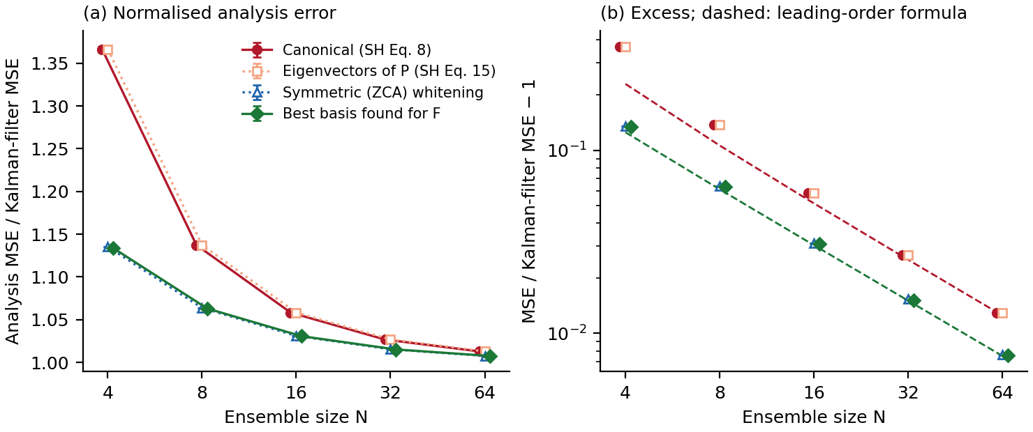
| Ensemble size $N$ | Canonical | ZCA whitening | Best basis found | Excess error removed (best found) |
|---|---|---|---|---|
| 8 | 1.137 | 1.064 | 1.063 | 54% |
| 16 | 1.058 | 1.031 | 1.031 | 47% |
| 32 | 1.027 | 1.015 | 1.015 | 43% |
| 64 | 1.013 | 1.008 | 1.008 | 42% |
Analysis error as a multiple of the Kalman-filter error (ensemble-mean update), from the paper's Table 6.
What it assumes. The coordinates are built from the true (oracle) forecast covariance; the analysis is a single step; the ensemble is Gaussian; localisation uses fixed tapers. When the coordinates are instead estimated from small pilot samples, much less of the gain survives, and heavy regularisation reverses it.
Summary for specialists
One analysis with prior $x\sim N(0,P)$, $P=LL^{\mathsf T}$, observation $y=Hx+\varepsilon$, $\varepsilon\sim N(0,R)$, and an independent Gaussian ensemble of size $N$ ($\nu=N-1$). Loss $(\hat x-x)^{\mathsf T}\Omega(\hat x-x)$ with whitened weight $W=L^{\mathsf T}\Omega L$: physical loss $\Omega=I$, prior-normalised loss $\Omega=P^{-1}$ ($W=I$). With $G$ the whitened observation operator, $C=(I+G^{\mathsf T}G)^{-1}$, $B=I-C$ and $A=CWC$. Complete localisation in an orthonormal whitened basis $U=[u_1,\dots,u_m]$ keeps only the sample variances; canonical tapers are deterministic symmetric Schur multipliers in canonical coordinates.
| Result | Content | Status |
|---|---|---|
| Lemma 3.1 | Complete localisation is the best canonical taper with unit observed diagonal (zero-correlation case of Flowerdew, 2015) | Proof |
| Theorem 3.3, Corollary 3.4 | Scalar observation, physical loss, every $N\ge2$: if $H^{\mathsf T}$ is not an eigenvector of $P$, a small rotation plus complete localisation beats every canonical taper with unit observed diagonal | Proof |
| Theorem 3.7 | With the same rescaling $\operatorname{diag}(\tau_0,1,\dots,1)$ in the rotated basis, the rotation beats every canonical taper with any observed-variance factor $\tau>0$; an unrescaled rotation need not (Remark 3.8) | Proof |
| Section 4.1, Appendix A | Two-dimensional example: explicit rational rotation with risk gap $\le-1/20416536$ at $N=3$ | Proof + exact arithmetic |
| Proposition 4.1 | Aligned example: canonical basis a strict local maximum of the risk at $N=3$ | Proof + exact; other $N$ numerical |
| Proposition 5.1, Corollaries 5.2–5.3 | Several observations, any $N$, against rotated complete localisations: not stationary if the loss couples an observed and an unobserved canonical direction; stationary if $[W,C]=0$ | Proof |
| Conjecture 5.4 | Sign property for two observed directions (would make $[W,C]=0$ necessary and sufficient) | Numerical only |
| Theorem 6.1 | Uniform expansion; leading basis-dependent term $2F(U)/\nu$ with remainder $O(\nu^{-3/2})$ | Proof |
| Theorem 7.1 | Canonical coordinates minimise $F$ iff $[A,B]=0$ and the eigenvalues are oppositely ordered | Proof |
| Corollary 7.6 | If the criterion fails, canonical tapers are beaten for all large $N$ | Proof |
| Proposition 8.1 | $W=I$, scalar observation, finite $N$: strict local minimum modulo completion if $\zeta>0$, not a local minimum if $\zeta<0$ | Proof; $\zeta>0$ numerical (Open problem 8.2) |
| Section 10, Corollary 10.1 | Testbed reconstruction; Fourier bases under physical loss are not leading-order optimal when two modes have prior variance below the observation-error variance | Numerical; corollary proved |
The leading objective is
uniformly over orthonormal $U$, for the ensemble-mean update (for the known-mean update the $\operatorname{tr}(WC^2)/N$ term is absent). Canonical coordinates diagonalise $B$; they minimise $F$ exactly when $[A,B]=0$ and, in a common eigenbasis, $(\lambda_i-\lambda_j)(\mu_i-\mu_j)\le0$ for the eigenvalues $\lambda_i$ of $A$ and $\mu_i$ of $B$ (Theorem 7.1). Under $W=I$, $A=C^2$ and the criterion always holds, so canonical coordinates are leading-order optimal among complete localisations and unit-diagonal positive semidefinite tapers in whitened bases (Remark 7.5).
Technical account
Why rotation helps (Section 3). In canonical coordinates the observed direction carries all the information, and complete localisation keeps its noisy sample variance $D\sim\chi^2_\nu/\nu$. The first variation of the risk under a rotation in the plane of the observed direction and another direction $j$ is $2\beta W_{1j}\gamma_{\nu,a}$ with $\gamma_{\nu,a}=\mathbb E[(D-1)(D-a)/(1+\beta D)^2]>0$ (Theorem 3.3). Under physical loss $W_{1j}\ne0$ precisely when $H^{\mathsf T}$ is not an eigenvector of $P$, so a small rotation of the right sign strictly lowers the risk. Lemma 3.1 shows complete localisation is already the best canonical taper with unit observed diagonal, so the rotation beats them all. The inflation results replace $D$ by $\tau D$; a monotone-likelihood-ratio argument and a Stein identity locate the best $\tau$, and the same derivative argument goes through with matched rescaling.
Certificates (Section 4). For $P=\begin{pmatrix}1&1\\1&2\end{pmatrix}$, $H=(1,0)$, $R=1$, an explicit rational rotation ($t=1/972216$) gives the exact risk gap $\mathcal R_3(Q)-\mathcal R_3(I)\le-1/20416536$ at $N=3$, certified with rational arithmetic and an explicit second-derivative bound $H_0=23148$. In an aligned example, a polynomial certificate $460/773$ gives curvature bounds $-56/773$ and $-508/773$, making the canonical basis a strict local maximum at $N=3$.
Several observations (Section 5). The first variation for any observation matrix is an explicit sum over pairs of canonical directions. A loss coupling between an observed and an unobserved direction gives a nonzero term for every $N$; commutation $[W,C]=0$ makes every term vanish.
Large ensembles (Sections 6–7). A uniform expansion of the risk, with explicit gain-derivative, moment and tail bounds and a Schur-multiplier norm bound, isolates $F(U)$. The criterion of Theorem 7.1 follows from the classical trace inequality for oppositely ordered (antimonotone) pairs of commuting matrices, credited to Bourin (1999) and Fujii (2005) and not claimed here; every canonical basis has $F=\operatorname{tr}(AB)$. A two-by-two example (Remark 7.2) shows physical loss alone does not condemn canonical coordinates: the criterion decides.
Prior-normalised loss at finite $N$ (Section 8). For $W=I$ and a scalar observation the canonical basis is stationary; its second variation reduces to the sign of one scalar $\zeta_{\nu,a,\beta}$, positive in every case computed (minimum ratio 1.0020 on the grid) but unproved.
Testbed (Section 10). 200 grid points, 50 point observations, a Matérn-type prior covariance with unit variance and unit observation-error variance, tuned to Snyder and Hakim's stated correlation length. The best basis found minimises $F$ by Riemannian descent from ZCA; it is a best value found, not a certified optimum.
Classical and new. The trace inequality, Wishart moments and the Schur-product setting are classical, and Lemma 3.1 is the zero-correlation case of Flowerdew (2015). Furrer and Bengtsson (2007) earlier gave a taper of the same form under a covariance-error criterion, showed by Jensen's inequality that the sample gain is biased low, and expanded the error of the analysis covariance in a fixed eigenbasis. They do not optimise over bases, and their expansion is not the risk expansion here. New, as far as a bounded literature search found, are the all-$N$ counterexamples, the inflation-robust version, the exact certificates, the vector-observation obstruction, the leading objective with its sharp criterion, the finite-$N$ prior-normalised reduction and the testbed comparison. A bounded search cannot establish priority.
Evidence, assurance and limitations
The synthetic audio briefing is explanatory, not additional evidence. Its complete transcript is available for reading.
- Proofs. Written out in full in the 31-page paper; not machine-verified. Conjecture 5.4 and Open problem 8.2 are numerical only, and the $O(\nu^{-2})$ remainder is a sketch.
- Exact arithmetic.
exact_certificates.pychecks the finite constants used in the proofs with Python fractions: 37 checks, including 4 negative controls that must fail. - Floating-point checks.
numerical_checks.py(82 checks, deterministic quadrature),theory_checks.py(296 checks, including a seeded Monte Carlo of the actual ensemble procedure with $4\times10^6$ ensembles and negative controls) andsh_testbed.py(39 checks, the testbed). These are consistency checks and illustrations, not interval certificates. - Replay. All four scripts were rerun from a fresh copy of the package with Python
-I -Band with-O(CPython 3.11.14, NumPy 2.3.5, SciPy 1.17.0, Matplotlib 3.10.8, mpmath 1.4.1). All passed, every recorded value matched the shipped results apart from timings and version strings, and the figures were byte-identical. The scripts contain noassert, so-Ocannot switch checks off. GitHub CI on Linux reruns all four in both modes. - Review. Internal AI-assisted review only: five reviewer roles, a separate-model adversarial review, one revision round with extensions, a proof audit and a separate-model audit of the new proofs, and a re-review. No reviewer found an error in a stated result; wording was tightened where claims were broader than the proofs. None of this is human peer review, independent reproduction or formal verification.
- Scope. One analysis step; independent Gaussian ensemble; oracle prior covariance used to build every basis; deterministic tapers. Not covered: cycling, model error, sample-adaptive localisation, shrinkage, hybrid covariances, tuned distance-based localisation, operational data and the regime of far more variables than members. With several observations the finite-$N$ result compares only with rotated complete localisations.
- Testbed. A reconstruction from Snyder and Hakim's text, not a replication of their figures. Bases estimated from small pilot samples keep much less of the gain.
Who should care, and why
| Audience | Potential use | Required caution |
|---|---|---|
| Ensemble data-assimilation developers | Choose the coordinates for localisation with the loss in mind: use $F(U)$, or simply symmetric whitening, instead of canonical coordinates when error is scored in physical units | Oracle prior covariance; one Gaussian analysis step; estimated bases are fragile |
| Theorists of localisation and sampling error | A sharp leading-order criterion, exact finite-$N$ counterexamples and a reduction of the prior-normalised case to one inequality | $\zeta>0$ and Conjecture 5.4 are open |
| Statisticians working on whitening and covariance estimation | A worked case where ZCA whitening beats the decorrelating canonical (SVD) transform for a downstream estimation risk | Specific to this risk and setting |
| Research agents | Claim map, agent index and replayable exact and numerical checks | Checks corroborate; results rest on the written proofs |
Why the problem matters
Covariance localisation is essential to every ensemble data-assimilation system, and choosing the variables in which to localise is a live design question. Snyder and Hakim offered an elegant, principled answer. This paper shows that the answer is right for one natural error measure and wrong for the one used in practice and in their own experiments, and it gives a computable rule for telling the two apart.
How to inspect or reproduce the recorded checks
From the GitHub release or the Zenodo archive, in the package root (each script refuses to overwrite an existing --out directory):
shasum -a 256 -c MANIFEST.sha256
uv run --with numpy==2.3.5 --with scipy==1.17.0 --with matplotlib==3.10.8 --with mpmath \
  python3 -I -B scripts/exact_certificates.py --out rerun/exact_certificates
uv run --with numpy==2.3.5 --with scipy==1.17.0 --with matplotlib==3.10.8 --with mpmath \
  python3 -I -B scripts/numerical_checks.py --out rerun/numerical_checks
uv run --with numpy==2.3.5 --with scipy==1.17.0 --with matplotlib==3.10.8 --with mpmath \
  python3 -I -B scripts/theory_checks.py --out rerun/theory_checks
uv run --with numpy==2.3.5 --with scipy==1.17.0 --with matplotlib==3.10.8 --with mpmath \
  python3 -I -B scripts/sh_testbed.py --out rerun/sh_testbed
The four runs take about three minutes in total, single-threaded. VERIFICATION.md maps each claim to its proof and check, AI_INDEX.md gives a machine-oriented claim map, and REVIEW_SUMMARY.md lists the review objections and their resolution.
The most valuable next projects
- Prove $\zeta>0$ (Open problem 8.2) and decide whether canonical localisation is globally optimal at finite $N$ under prior-normalised loss.
- Prove the two-observation sign conjecture (Conjecture 5.4).
- Find a data-driven, loss-aware basis that is robust to misestimated small prior variances.
- Test whether the one-step advantage persists in a cycling filter with a propagated ensemble covariance.
- Optimise the basis and a partial taper jointly, including inflation.
- Develop the analogue of $F$ when the number of variables grows with the ensemble.
What is in the evidence package
The 31-page paper (PDF and LaTeX source) with two figures; the bibliography with the script that generates it from Crossref records; four verification scripts with their recorded outputs; a claim-by-claim verification ledger; an agent index; a dated record of the prior-art scrutiny; a rating-free review summary and pre-revision development notes. Licences (text, figures and data CC0-1.0; code MIT), citation metadata, CI and SHA-256 sums for every file. The paper is an unrefereed candidate, released for scrutiny.
Verification status
Unrefereed AI-assisted mathematics candidate. The main results have written proofs; Conjecture 5.4 (two observed directions) and Open problem 8.2 (the prior-normalised finite-N inequality) are supported numerically only; the testbed is a numerical reconstruction, not a replication. Internal AI-assisted review in five roles, a separate-model adversarial review, one revision round with extensions, a proof audit and separate-model audit of the new proofs, and a re-review. No human peer review, independent reproduction or formal verification has been established.
Cite
BibTeX
@misc{canonicalcovariancelocalisationfailure2026,
  title        = {When canonical covariance localisation fails},
  author       = {Anonymous},
  year         = {2026},
  doi          = {10.5281/zenodo.23941881},
  url          = {https://doi.org/10.5281/zenodo.23941881},
  version      = {0.2.0-candidate},
  howpublished = {Zenodo},
  note         = {Unrefereed; internally replayed evidence package. Press page: https://evidencepress.org/releases/canonical-covariance-localisation-failure/}
}Also: cite.bib · paper.json · this page as Markdown